This tutorial provide the basics on time series analysis.

• Python
• Time Series

In this tutorial we provide some basics on time series so you can go further exploring different types of time series problems. It will serve as base to understand the forecasting algorithms that will be introduced in future tutorials.

The complete code of this tutorial can be found at 01-Intro_time_series_tutorial.ipynb on GitHub.

After completing this tutorial, you will know: 

1. How to decompose time series 
2. How to identify time series properties
3. The importance of stationarity
4. How to make a time series stationary

Introduction to Time Series

Time series analysis deals with data that is ordered in time. Time series data is one of the most common data types and it is used in a wide variety of domains: finance, climate, health, energy, governance, industry, agriculture, business etc. Being able to effectively work with such data is an increasingly important skill for data scientists, especially when the goal is to report trends, forecast, and even detect anomalies.

The current explosion of Internet of Things (IoT)  – that collects data using sensors and other sources –  allows industries to use anomaly detection to predict when a machine will malfunction. This permits taking action in advance and avoid stopping production. However, this is an example of anomaly detection, which won’t be the main focus of this tutorial. Our main focus is to introduce time series and include some time series forecasting methods.

Some examples where time series are used as forecasting methods include:

• Public Administration: By forecasting the consumption of water and energy for the next years, governments are able to plan and build the infrastructure necessary avoiding collapse in the distribution of these resources.
• Health: Hospitals can use historical data to know the number of intensive care units necessary in the future, or even plan the number of nurses per shift in order to reduce the waiting time on emergency rooms.
• Different type of businesses: Analysing business trends, forecasting company revenue or exploring customer behaviour. 

All in all, no matter which application, there is a great interest in the use of historical data to forecast demand so we can provide consumers what they need without wasting resources. If we think about agriculture, for example, we want to be able to produce what people need without harming the environment. As a result, we are not only having a positive impact on the life producers and consumers but also on the life of the whole society.

These few examples already give a good idea of why time series are important and why a data scientist should have some knowledge about it.

Components of Time Series and Time Series Properties

Time Series Decomposition

In general, most time series can be decomposed in three major components: trend, seasonality, and noise. 

• trend shows whether the series is consistently decreasing (downward trend), constant (no trend) or increasing (upward trend) over time.
• seasonality describes the periodic signal in your time series. 
• noise or residual displays the unexplained variance and volatility of the time series.

We can easily access those components applying Python’s statsmodels library seasonal_decompose.

Time Series Properties

Time series components help us recognizing some of important properties such as seasonality, cyclicality, stationarity, and whether the time series is additive or multiplicative.  Throughout this tutorial, you will learn how recognizing and understanding such properties is essential in the process of building a successful forecasting model.

Seasonality x Cyclicality

By observing the seasonal component, we can say if the time series is seasonal or cyclic. Seasonality should always present a fixed and known period. If there is no fixed or known period, we are observing a cyclic signal, i.e., cyclicality.

Stationarity

A time series is stationary if its statistical properties do not change over time.

Many algorithms such as SARIMAX models are built on this concept. For those algorithms it is important to identify this property. This happens because when running linear regression, the assumption is that all of the observations are independent of each other. In a time series, however, we know that observations are time dependent. So, by making the time series stationary we are able to apply regression techniques to time dependent variables. In other words, the data becomes easier to analyse over long periods of time as it won’t necessarily keep varying and so, the algorithms can assume that stationary data and make better predictions.

If the time series is non-stationary there are ways to make it stationary.

A stationary time series fulfills the following criteria:

1. The trend is zero.
2. The variance in the seasonality component is constant: The amplitude of the signal does not change much over time.
3. Autocorrelation is constant: The relationship of each value of the time series and its neighbors stays the same.

In addition, to analyzing the components a common way to check for stationarity is to apply statistical tests such as the Augmented Dicky-Fuller test (ADF) and the Kwiatkowski-Phillips-Schmidt-Shin test (KPSS). Both tests are part of the Python statsmodel library. In the Example’s section we give more details about these tests and how to apply them.

Additive x Multiplicative Model

As seen previously a time series is a combination of its components: trend, seasonal, and residual components. This combination can occur either in an additive or multiplicative way.

Additive Model

In an additive model these components are added in linear way where changes over time are consistently made by the same amount.

In the decomposition we can identify it by:

• Linear trend: Trend is a straight line
• Linear seasonality: Seasonality with same frequency (width of cycles) and amplitude (height of cycles).

Multiplicative Model

On the other side, in a multiplicative model, components are multiplied together:

Therefore, this model is nonlinear (e.g., quadratic or exponential) and changes increase or decrease over time.

• Non-linear trend: trend is a curved line
• Non-linear seasonality: Seasonality varies in frequency (width of cycles) and/or amplitude (height of cycles).

One of the main objectives for a decomposition is to estimate seasonal effects that can be used to create and present seasonally adjusted values. 

So to choose between additive and multiplicative decompositions we consider that:

• The additive model is useful when the seasonal variation is relatively constant over time.
• The multiplicative model is useful when the seasonal variation increases over time.

Now time to put all this together and analyse some time series.

Example of Time Series

Google Trends Data

Consider the search for the word “Diet” from the week starting at 2016-03-27 till week starting at 2021-03-21. The dataset is available here.

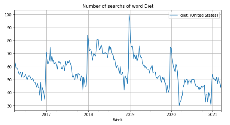
The plot above shows a clear pattern: At the end of the year the word Diet has the lowest number of searches while at the beginning of the year it has the highest number of searches. Do people at the end of the year just want to celebrate and enjoy good food? In consequence, do they choose as New Year’s resolution to become in good shape?

This time series has a seasonal pattern, i.e., it is influenced by seasonal factors. Seasonality occurs over a fixed and known period (e.g., the quarter of the year, the month, or day of the week). In this case the period seems to be yearly and causes a peek at the festivities at the end of year.

We can also observe that there is no constant increase or decrease in trend which would suggest a non-linear trend.

Let’s decompose this time series in its components. Because we believe that trend is non-linear, we will set parameter model as multiplicative. By default, this parameter is additive.

Parameter period is optional but you can set it depending on the time series. Because the data is given in weeks, we set the parameter period to the the number of weeks in a year.

	import statsmodels.api as sm
	decomposition = sm.tsa.seasonal_decompose(diet[‘diet: (United States)’],
	model = ‘multiplicative’,
	period=53 #52 to 53 weeks in a year
	)
	fig = decomposition.plot()
	plt.show()

view rawdecompose_mult.py hosted with ❤ by GitHub

Observe that both frequency and amplitude of seasonal component do not change with time suggesting linear seasonality, i.e., a seasonal additive model. Let’s change parameter model to additive.

As we suspected, the trend is non-linear. More than this, the time series follows no consistent upwards or downwards slope. Therefore, there is no positive (upwards slope) or negative (downwards slope) trend.

Also, if we compare multiplicative and additive residuals, we can see that the later is much smaller. As a result, a additive model (Trend + Seasonality) fits the original data much more closely.

Want to know more? Check this interesting article about performing additive and multiplicative decomposition.

Stationarity Tests 

Augmented Dicky-Fuller test (ADF) is a very popular test for stationarity. However, it can happen that a time series passes the ADF test, without being stationary. Kwiatkowski-Phillips-Schmidt-Shin (KPSS) is another test for checking the stationarity of a time series. It is prudent to apply both tests, so that it can be ensured that the series is truly stationary. Next to that, we cannot forget the importance of also observing the time series plot.

ADF test

ADF test is used to determine the presence of unit root in the series, and hence helps in understanding if the series is stationary or not. The null and alternate hypothesis of this test are:

Null Hypothesis: The series has a unit root, meaning it is non-stationary. It has some time dependent structure.

Alternate Hypothesis: The series has no unit root, meaning it is stationary. It does not have time-dependent structure.

If the null hypothesis failed to be rejected, this test may provide evidence that the series is non-stationary.

A p-value below a threshold (such as 5% or 1%) suggests we reject the null hypothesis (stationary), otherwise a p-value above the threshold suggests we fail to reject the null hypothesis (non-stationary).

KPSS test

The null and alternate hypothesis for the KPSS test is opposite that of the ADF test.

Null Hypothesis: The process is trend stationary.

Alternate Hypothesis: The series has a unit root (series is not stationary).

A p-value below a threshold (such as 5% or 1%) suggests we reject the null hypothesis (non-stationary), otherwise a p-value above the threshold suggests we fail to reject the null hypothesis (stationary).

The following functions can be found here. 

	from statsmodels.tsa.stattools import adfuller
	def adf_test(timeseries):
	print (‘Results of Dickey-Fuller Test:’)
	dftest = adfuller(timeseries, autolag=’AIC’)
	dfoutput = pd.Series(dftest[0:4], index=[‘Test Statistic’,’p-value’,’#Lags Used’,’Number of Observations Used’])
	for key,value in dftest[4].items():
	dfoutput[‘Critical Value (%s)’%key] = value
	print (dfoutput)

view rawadf_test.py hosted with ❤ by GitHub

	from statsmodels.tsa.stattools import kpss
	def kpss_test(timeseries):
	print (‘Results of KPSS Test:’)
	kpsstest = kpss(timeseries, regression=’c’, nlags=”auto”)
	kpss_output = pd.Series(kpsstest[0:3], index=[‘Test Statistic’,’p-value’,’Lags Used’])
	for key,value in kpsstest[3].items():
	kpss_output[‘Critical Value (%s)’%key] = value
	print (kpss_output)

view rawkpss_test.py hosted with ❤ by GitHub

When applying those tests the following outcomes are possible:

Case 1: Both tests conclude that the series is not stationary – The series is not stationary.

Case 2: Both tests conclude that the series is stationary – The series is stationary.

Case 3: KPSS indicates stationarity and ADF indicates non-stationarity – The series is trend stationary. The trend needs to be removed to make the time series strict stationary. After that, the detrended series is checked for stationarity.

Case 4: KPSS indicates non-stationarity and ADF indicates stationarity – The series is difference stationary. Differencing is used to make the series stationary. After that, the differenced series is checked for stationarity.

Let’s apply the tests on the Google Trends data.

Based upon the significance level of 0.05 and the p-value:

ADF test: The null hypothesis is rejected. Hence, the series is stationary

KPSS test: There is evidence for rejecting the null hypothesis in favour of the alternative. Hence, the series is non-stationary as per the KPSS test.

These results fall in case 4 of the above mentioned outcomes. In this case, we should apply differencing to make the time series stationary and again apply the tests until we have both tests pointing to stationarity.

Summing up, the analysis made for the Google dataset so far shows that:

1. The trend is non-linear (multiplicative) and is not increasing or decreasing all the time.
2. We have seasonality, which apparently is influenced by end-of-the-year festive period.
3. Seasonality is linear, i.e., seasonality does not vary in frequency (width of cycles) neither amplitude (height of cycles).
4. Additive residuals are smaller than multiplicative residuals.
5. Time series is stationary according to ADF test, but not according to KPSS test. Therefore, we need differencing to make the time series stationary.

Because of the linear seasonality and small additive residuals we can conclude that an additive model is more appropriate in this case.

Making Time Series Stationary

Many statistical models require the time series to be stationary to make effective and precise predictions. This is the case of ARIMA models which we will see in 02-Forecasting_with_SARIMAX.ipynb.

A very common way to make a time series stationary is differencing: from each value in our time series, we subtract the previous value. 

Other transformations can also be applied. We could, for instances, take the log, or the square root of a time series.

	def obtain_adf_kpss_results(timeseries, max_d):
	“”” Build dataframe with ADF statistics and p-value for time series after applying difference on time series
	Args:
	time_series (df): Dataframe of univariate time series
	max_d (int): Max value of how many times apply difference
	Returns:
	Dataframe showing values of ADF statistics and p when applying ADF test after applying d times
	differencing on a time-series.
	“””
	results=[]
	for idx in range(max_d):
	adf_result = adfuller(timeseries, autolag=’AIC’)
	kpss_result = kpss(timeseries, regression=’c’, nlags=”auto”)
	timeseries = timeseries.diff().dropna()
	if adf_result[1] <=0.05:
	adf_stationary = True
	else:
	adf_stationary = False
	if kpss_result[1] <=0.05:
	kpss_stationary = False
	else:
	kpss_stationary = True
	stationary = adf_stationary & kpss_stationary
	results.append((idx,adf_result[1], kpss_result[1],adf_stationary,kpss_stationary, stationary))
	# Construct DataFrame
	results_df = pd.DataFrame(results, columns=[‘d’,’adf_stats’,’p-value’, ‘is_adf_stationary’,’is_kpss_stationary’,’is_stationary’ ])
	return results_df

view rawobtain_adf_kpss_results.py hosted with ❤ by GitHub

You can’t see any trend, or any obvious changes in variance, or dynamics. This time series now looks stationary.

Visit notebook 01-Intro_time_series_tutorial.ipynb on GitHub for one more example using global temperature dataset time series. This dataset includes global monthly mean temperature anomalies in degrees Celsius from 1880 to the present. Data are included from the GISS Surface Temperature (GISTEMP) analysis and the global component of Climate at a Glance (GCAG).

Conclusions

In this tutorial you were introduced to time series. You’ve learnt about important time series properties and how to identify them using both statistical and graphical tools.

In the future tutorials we will use what was learnt so far and be introduced to some forecasting algorithms:

• SARIMAX models
• Facebook Prophet